Interpolating with implicit modeling
Written by nTop
Published on April 12, 2019
The last two posts in this implicit modeling series introduced the implicit representation and how it enables failure-proof, simple operations like offsets and booleans. To get a better understanding of the power of implicits and a more intuitive feel for how they work, let’s look at a series of interpolation operations on two shapes.
Loft-like blending
In the simplest implementation, one can interpolate distance fields to create loft-like geometry between profiles of arbitrary topology and complexity. Here’s a simple example:
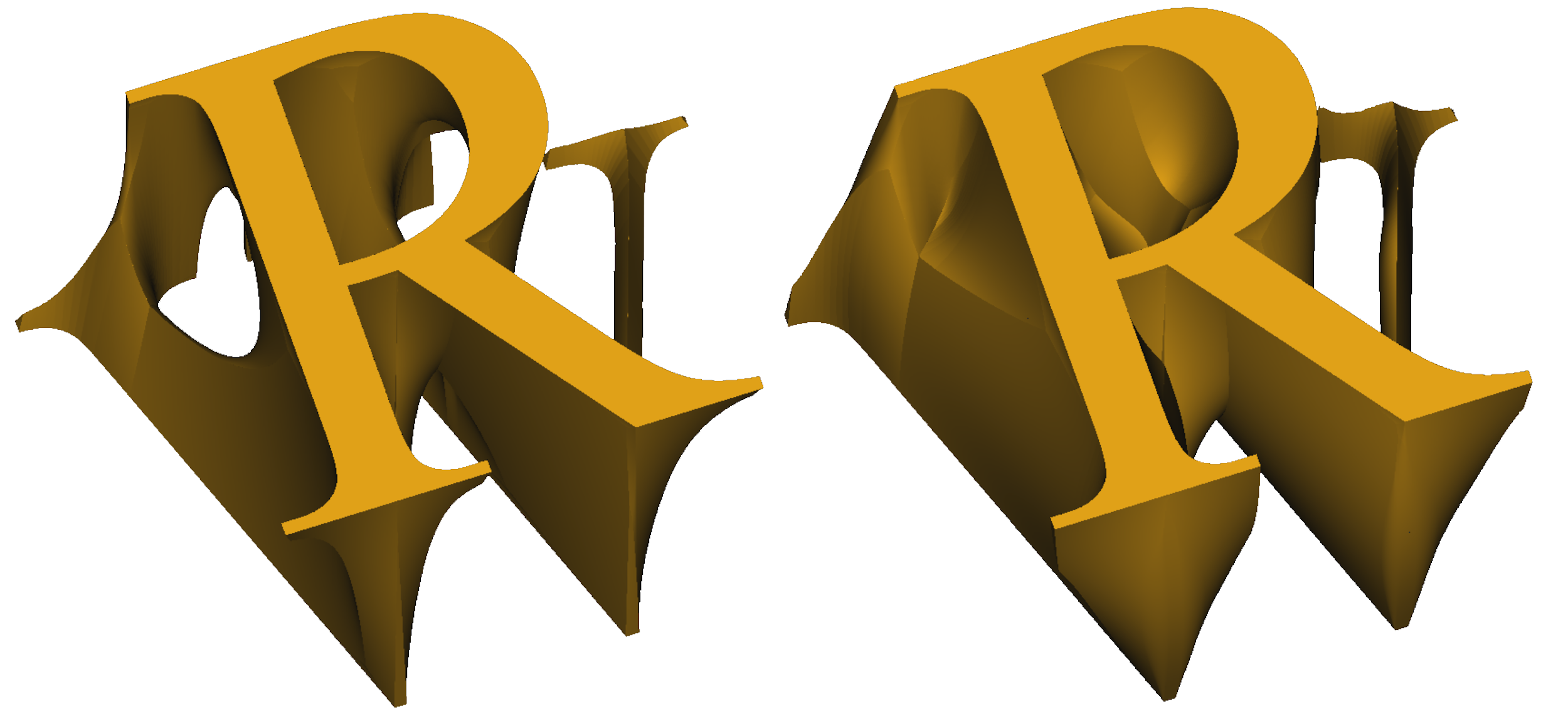
An implicit blended loft between an uppercase R and a W. The example on the left shows simple interpolation, while the right adds a bulge via a variable offset.
With implicits, a blended loft is just the linear interpolation of any two shapes, regardless of complexity or topology. One can perform the loft while sweeping or by overlapping two bodies simply by interpolating over a function of space. If we call our two implicits R and W, the interpolation is produced by a function we’ll call, “mix(R, W, t),” where t’s domain is from 0 to 1 and mix is defined by:
- mix(R, W, t) = (1-t) * R + t * W
In the example above, the range of t was mapped from the bottom to the top of two extrusions, but they could just as easily be mapped in another direction or using a more complicated function.
To add more material in the center, as shown on the right, we can add extra offset using another function of t:
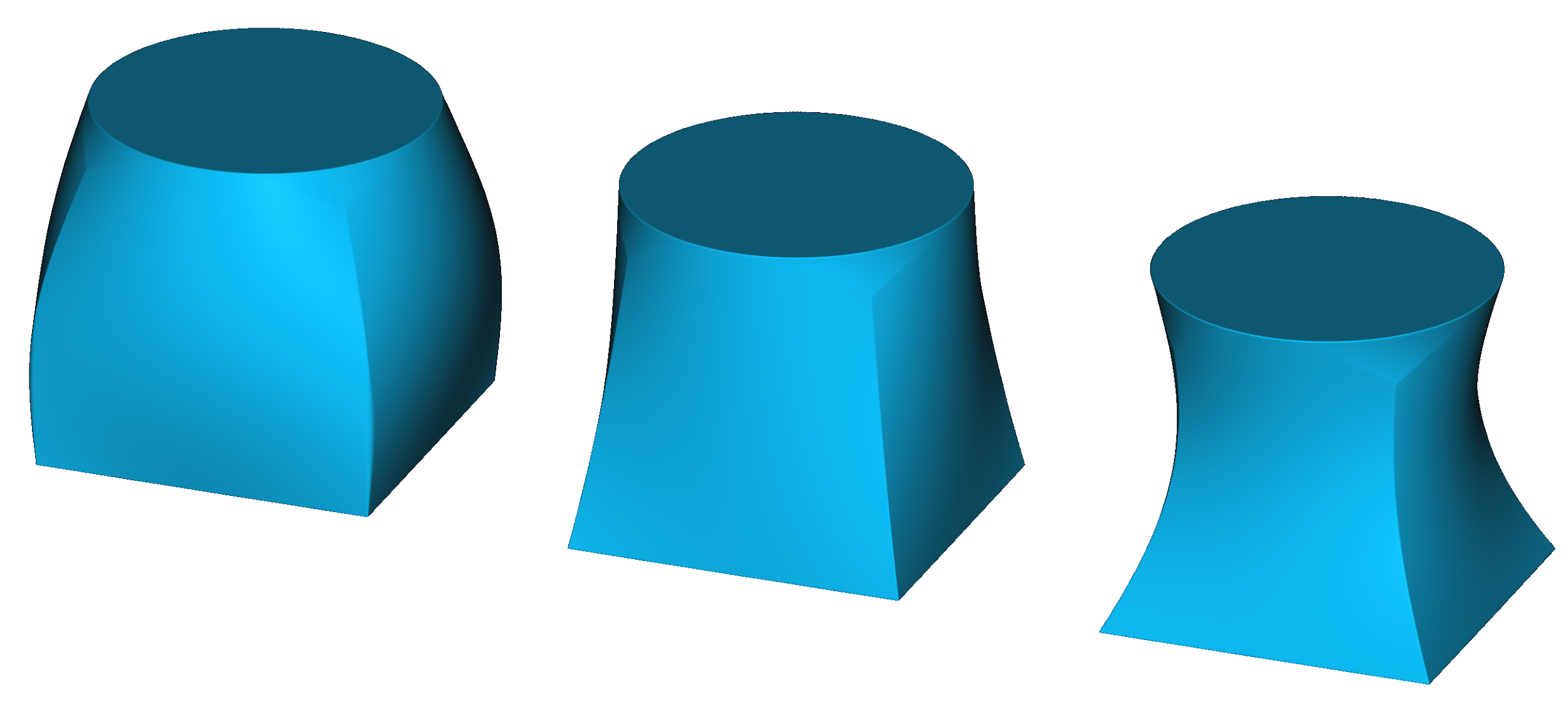
A blended loft between a cylinder and a box with an outward, zero, and inward bulge.
A bulge can be modeled by any curve. In order to preserve the starting and ending sections, the curve should be zero at t = 0 and 1. The sine function proves convenient:
- mix(R, W, t) - a * sin(π * t)
Where a is the amount of outward bulge desired.
Morphing
Above, we used the variable t to vary spatially. By keeping it constant in space, we can create a linear combination of two different models. We can animate looping t back and forth:
Interpolating between R and W, animated through time. The entire 3D shape is being morphed, causing 3d effects near the top and bottom.
In the universe of mechanical design, we don’t see many parts that change shape quite this dramatically. However, there are some useful applications of morphing in manufacturing processes like forging design, where a part needs to be transformed at constant volume from one shape to another in a series of pressings.
Midsurfacing
Let’s examine what two implicits look like when they overlap, observing one line of distance values across two shapes and comparing those fields:
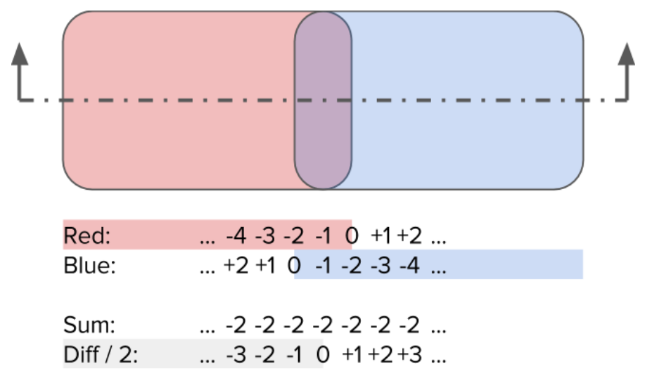
The 1D section of two overlapping 2D shapes shows the underlying distance values for each shape. Notice that the sum is a measurement of local clearance or interference, and the difference (normalized) produces an implicit of the midsurface.
What do we mean by a midsurface? There are many CAE and CAM applications, such as FEA using shell elements and sheet metal manufacturing, where one might want to construct a surface that represents the halfway point between two surface or solid bodies. Due to the difficulty of extracting midsurfaces in traditional CAD, if midsurfaces are needed, the best practice is to design them first. What if you want to extract them post-facto, or are interested in computing a halfway surface between two complex parts?
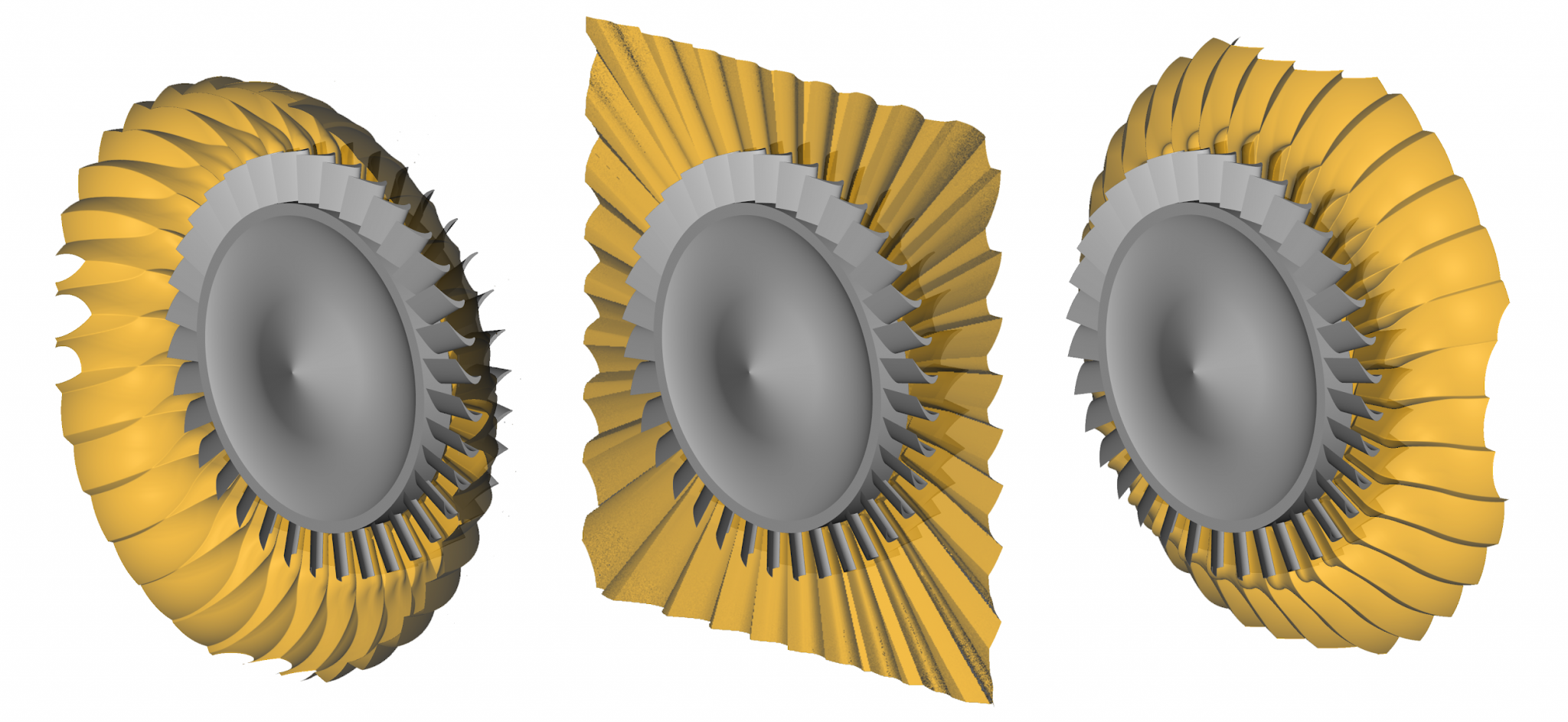
The t = 0.45, 0.5, and 0.55 midsurfaces between a rotor and stator with 33 and 34 blades, respectively, with the shroud removed so the midsurfaces demonstrate their natural extension. The surface was generated in nTop from CAD geometry derived from this turbojet model.
A midsurface is another kind of interpolation and is defined at any ratio of two shapes, but with one of the shapes inverted (implicit values negated), creating consistent direction to the implicit field for both shapes. Note that the inverted shape represents an inside-out part that extends off to infinity in all directions, and that the midsurfaces may partition space into separate, infinitely large regions. Therefore, implicit midsurfaces can have no natural bounds (an advantage over the spline geometry used in precise CAD) and can be smoothly and accurately evaluated as remotely as needed from the source models.
Interference removal
The idea of a midsurface is well defined both when parts have clearance or interference. By adding two fields, we produce a new field that locally measures the closest clearance or interference, as illustrated above. We can use that information to create clearance from overlapping parts in an assembly:
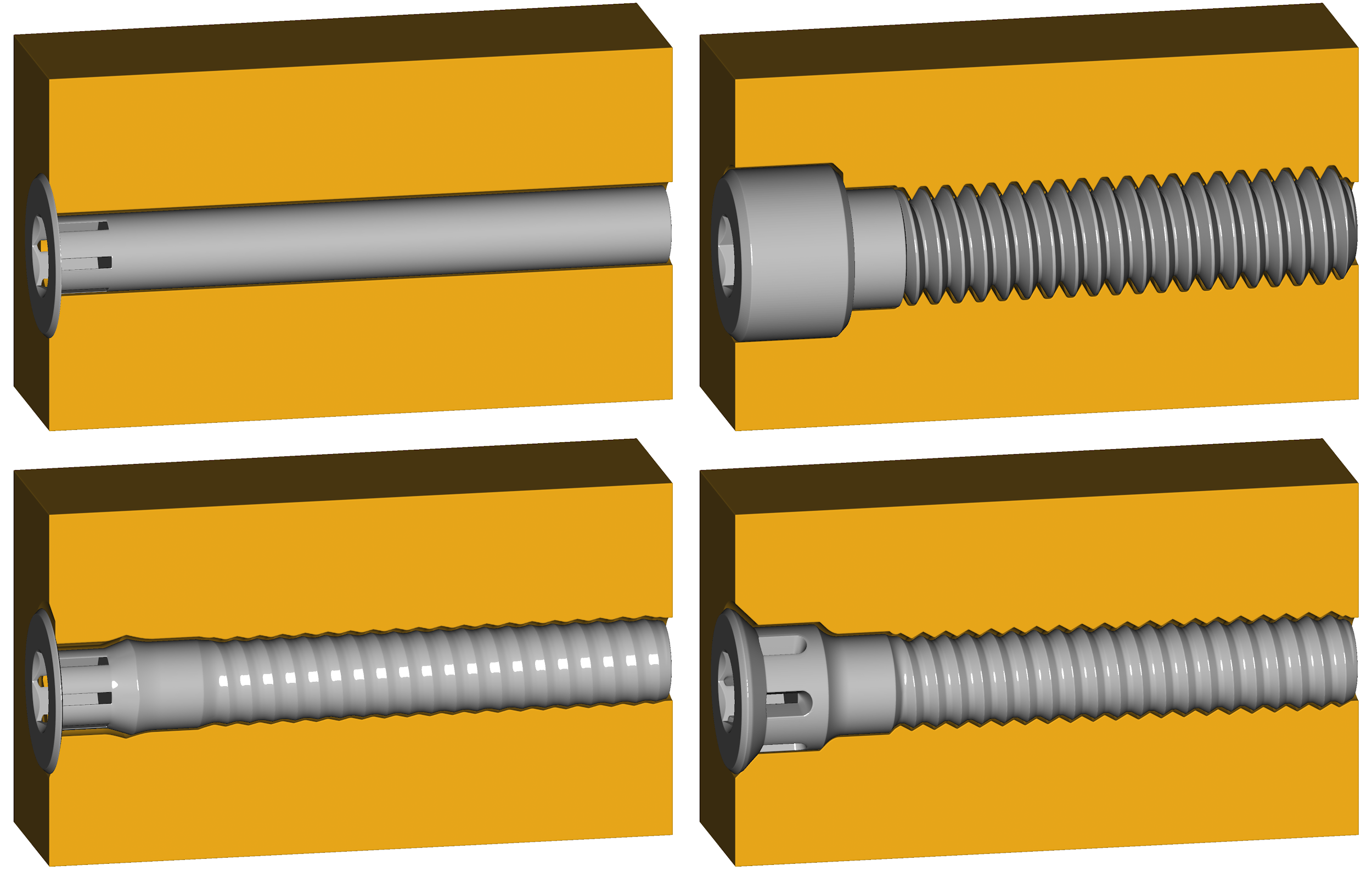
Clearance created between a block modeled only with a nominal tap hole and an overlaid cap screw. The top two images show one subtracted from the other with added clearance. The lower two images demonstrate that there exists a smooth range of interpolated options.
To create the clearance between two arbitrary parts, we’ll start with our midsurface as a function or our parameter, t.
- Midsurface = mix(A, -B, t)
At t = 0, Midsurface is equivalent to A, so this is the case where we would preserve A and offset B. Similarly, at t = 1, B should be preserved and A offset. That means how much we remove from each part should also be interpolated to give the desired gap:
- ClearanceA = t * Gap
- ClearanceB = (1-t) * Gap
We can now trim our original parts with an offset version of the midsurface to produce the new parts with added clearance, recalling that a boolean intersection is computed with max:
- A’ = max(A, ClearanceA + Midsurface)
- B’ = max(B, ClearanceB - Midsurface)
With only a few simple operations, we’re able to compute geometry operations that would be near-impossible to execute on B-reps. Finally, keep in mind that our ratio parameter, t, is a free parameter over space, so we can vary it anywhere we want, just like with the loft:
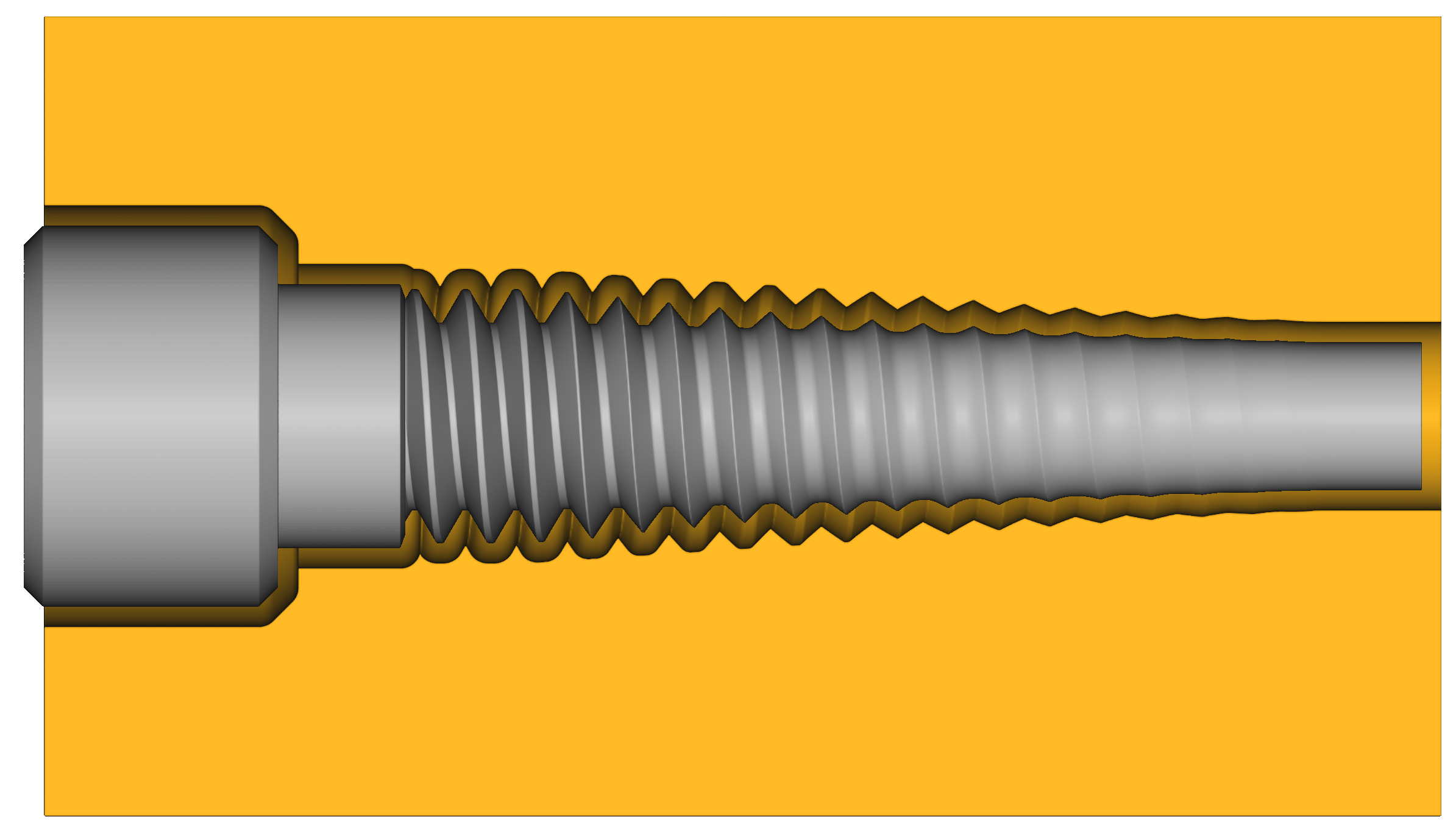
The same screw and hole, with the ratio parameter varying along the axis.
Interpolate everything
In this post, we covered how simple linear interpolation enables unprecedented versatility in lofting, morphing, midsurfacing and interference removal. This technique of simple interpolation also extends to extrapolation and non-linear functions for more advanced design and modeling applications. Combined with bulge-like interpolation control, these techniques provide a powerful new set of modeling capabilities.
This basic technique of interpolation also becomes an important methodology when using simulation data, lattices, and topology optimization to produce real parts. As we explore lightweighting, heat transfer, and fluid dynamic applications in upcoming posts, we’ll continue to use these interpolation techniques to create smooth transitions between domains. We’ll also see that even rounds or fillets can be thought of as a kind of interpolation.

nTop
nTop (formerly nTopology) was founded in 2015 with the belief that engineers’ ability to innovate shouldn’t be limited by their design software. Built on proprietary technologies that upend the constraints of traditional CAD software while integrating seamlessly into existing processes, nTop allows designers in every industry to create complex geometries, optimize instantaneously, and automate workflows to develop breakthrough parts and systems in record time.


